Southpaw
Well-Known Member
Introduction:
Zg requested that I look into the fluctuations that a counter could experience throughout their lifetime. As we all know, fluctuation in the game of blackjack is quite wild. We also know that the fluctuation tends to get smoothed out after a number of trials.
But can a lifetime provide enough trials to sufficiently smooth out the fluctuation that blackjack throws our way? I’ll examine this situation through a mathematical approach and a simulation-based approach.
Methodology:
Zg suggested that I assume a counter will get in 3-million rounds in a lifetime (100 hands per hour x 30 hours per week x 50 weeks per year x 20 years). Assuming that one plays 100 hands per hour, this represents 30,000 hours of play. He also suggested that I assume the counter uses a strong system, and that our counter has access to a pretty good double-deck game.
The Game I decided upon is of the following conditions:
2-Decks, H17, Split to 4, No RSPA, 3:2 BJ, DOA2, NS, 0.65 Pen, DAS, 1 other player, face-down (plays second)
The strong system that I decided the counter will use is HO2 (with ASC) and full-indices.
The spread Zg suggested was 1-2x4. I developed an optimal bet spread that assumed 1000 units bank and 13.5% RoR when playing with the above conditions. (Note that I had the spread set to 1-8 and just made the computer put out 2x4 instead of 1-8. 2x4 can technically be put out sooner than 1x8, but I ignored this.) Here is a summary of the spread:
https://docs.google.com/viewer?a=v&pid=explorer&chrome=true&srcid=0B0cCldUn36hMZTdiYzQxZDItNjM5Ny00NDZkLWE5NjYtOWE1MWI1MzhjMTcy&hl=fr
All simulations in this study have the following parameters:
Fixed Cut-Card, 1-Burn Card, Quarter-Deck Resolution, TC divisor = Cards in tray, Truncated TC, Rounded Deck Estimation.
The Mathematical Approach to the Problem:
I ran a simulation (400M rounds) with the above conditions and came up the following stats:
Win Rate per 100 rounds (per hour) = 2.19 units
Standard deviation per 100 rounds = 28.43 units
Some other stats that I won’t be using in calculations:
SCORE: $59.24
TBA: +1.031%
DI: 7.70
To solve this problem mathematically, I brushed up on my statistics and reread a portion of D.S.’s BJA. However, if any of my math is flagrantly incorrect, notify me immediately.
The “Expected Win” after “n” hours (100 rounds is 1 hour) = (Win Rate per hour) x (n hours)
The Standard Deviation after “n” hours = (Standard Deviation for 1 hour) x ((n hours)^½)
First, I’d like to find out one lifetime’s win rate plus or minus 1 standard deviation. After a lifetime (3 million rounds), one can expect to win (68.3% of the time):
(2.19 units per hour)(30,000 hours) +/- (28.43 units per hour)(30,000 hours)^(½) =
65,700 units +/- ~4,924 units
Expressed another way, 68.3% of the time our counter will earn between 60,776 and 70,624 units. Therefore, he has a 68.3% chance of earning between 2.03-2.35 units per 100 rounds (per hour).
Now, I’d like to find out one’s win rate plus or minus 2 standard deviations. After a lifetime (3 million rounds), one can expect to win (95.45% of the time):
(2.19 units per hour)(30,000 hours) +/- (2)(28.43 units per hour)(30,000 hours)^(½) =
65,700 units +/- ~9,848 units
Expressed another way, he has a 95.45% chance to earn between 55,852 and 75,548 units. Therefore, it follows that he has a 95.45% chance of earning between 1.86-2.52 units per 100 rounds (per hour).
Lastly, I’d like to find out one’s win rate plus or minus 3 standard deviations. After a lifetime (3 million rounds), one can expect to win (99.7% of time):
(2.19 units)(30,000 hours) +/- (3)(28.43 units per hour)(30,000 hours)^(½) =
65,700 units +/- ~14,772 units
Expressed another way, he has a 99.7% chance of earning between 50,928 and 80,472 units. Therefore, it follows that he has a 99.7% chance of earning between 1.70 and 2.68 units per 100 rounds (per hour).
The Simulation Approach to this Problem:
This portion of the study is actually what Zg had asked me to do. The mathematical approach taken above is something that I just decided to throw in. The mathematical approach can be used to reinforce the simulation approach.
Specifically, Zg asked me to run 100 3M round simulations and examine the distribution of results. This is exactly what I plan to do here. The parameters of these simulations are no different than the one described above, save for the fact that each simulation will only be 3M rounds, unlike the one above that was 400M rounds.
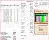
For each of the 100 completed simulations, I will report it’s hourly win-rate and will organize them moving from greatest to lowest (like the optimism of this organization?).
Results (this is just a list. If you'd like to see a graphical representation of the data, skip to the next link):
https://docs.google.com/viewer?a=v&pid=explorer&chrome=true&srcid=0B0cCldUn36hMMWJkZDM0N2YtZWIzOC00ZTBjLTkxNDctNTQ0ZGU1NWU2NmZi&hl=fr
Some Raw Stats:
Mean: 2.183 units per hour
Median: 2.170 units per hour
Minimum: 1.770 units per hour
Maximum: 2.530 units per hour
Here is a nice graphic summarizing the above data:
https://docs.google.com/viewer?a=v&pid=explorer&chrome=true&srcid=0B0cCldUn36hMNjU1MTU3ZTMtNjY5Ny00YzYwLTg0NDctNzFmMTFiMzczY2Y1&hl=fr
Conclusions:
I’ll leave that to you all.
Disclaimers:
The fluctuations that one might experience over 3,000,000 rounds are likely larger than depicted in this study for a few reasons. First of all, the game studied was a double-deck game. It is known that the ratio of win rate : Standard Deviation is significantly lower in shoe games than it is in double-deck games such as the one studied here. It may be unrealistic to assume that one can put in 30 hours per week at the DD tables for an extended period of time, for these games tend to be more uncommon than shoe games, and they tend to be watched a bit more closely by the pit. Because one would likely have to play the occasional shoe game, one’s lifetime win rate likely will have fluctuated away from their EV more greatly than this study may indicate.
Moreover, no one plays perfect. The strategy used in this study was HO2 with ASC, full-indices and quarter-deck resolution. If you try to implement a strategy this difficult, you WILL make an occasional “mistake,” however small or insignificant it may be. Mistakes tend to increase variance and / or lower your EV, neither of which is good for the counter.
Another reason that the typical counter can’t play perfect is the occasional need for cover. It is known that betting cover is quite pricey in terms of increasing variance and lowering EV, ESPECIALLY IN CASES WHERE ONE IS NOT GETTING VERY MANY ROUNDS PER SHOE (I.e., lower number of decks or more players at the table).
I could dabble on forever as to why one’s expected win rate will likely fluctuate even further than the study indicates, but I’d probably not mention anything that you’re not aware of.
Best,
SP
Zg requested that I look into the fluctuations that a counter could experience throughout their lifetime. As we all know, fluctuation in the game of blackjack is quite wild. We also know that the fluctuation tends to get smoothed out after a number of trials.
But can a lifetime provide enough trials to sufficiently smooth out the fluctuation that blackjack throws our way? I’ll examine this situation through a mathematical approach and a simulation-based approach.
Methodology:
Zg suggested that I assume a counter will get in 3-million rounds in a lifetime (100 hands per hour x 30 hours per week x 50 weeks per year x 20 years). Assuming that one plays 100 hands per hour, this represents 30,000 hours of play. He also suggested that I assume the counter uses a strong system, and that our counter has access to a pretty good double-deck game.
The Game I decided upon is of the following conditions:
2-Decks, H17, Split to 4, No RSPA, 3:2 BJ, DOA2, NS, 0.65 Pen, DAS, 1 other player, face-down (plays second)
The strong system that I decided the counter will use is HO2 (with ASC) and full-indices.
The spread Zg suggested was 1-2x4. I developed an optimal bet spread that assumed 1000 units bank and 13.5% RoR when playing with the above conditions. (Note that I had the spread set to 1-8 and just made the computer put out 2x4 instead of 1-8. 2x4 can technically be put out sooner than 1x8, but I ignored this.) Here is a summary of the spread:
https://docs.google.com/viewer?a=v&pid=explorer&chrome=true&srcid=0B0cCldUn36hMZTdiYzQxZDItNjM5Ny00NDZkLWE5NjYtOWE1MWI1MzhjMTcy&hl=fr
All simulations in this study have the following parameters:
Fixed Cut-Card, 1-Burn Card, Quarter-Deck Resolution, TC divisor = Cards in tray, Truncated TC, Rounded Deck Estimation.
The Mathematical Approach to the Problem:
I ran a simulation (400M rounds) with the above conditions and came up the following stats:
Win Rate per 100 rounds (per hour) = 2.19 units
Standard deviation per 100 rounds = 28.43 units
Some other stats that I won’t be using in calculations:
SCORE: $59.24
TBA: +1.031%
DI: 7.70
To solve this problem mathematically, I brushed up on my statistics and reread a portion of D.S.’s BJA. However, if any of my math is flagrantly incorrect, notify me immediately.
The “Expected Win” after “n” hours (100 rounds is 1 hour) = (Win Rate per hour) x (n hours)
The Standard Deviation after “n” hours = (Standard Deviation for 1 hour) x ((n hours)^½)
First, I’d like to find out one lifetime’s win rate plus or minus 1 standard deviation. After a lifetime (3 million rounds), one can expect to win (68.3% of the time):
(2.19 units per hour)(30,000 hours) +/- (28.43 units per hour)(30,000 hours)^(½) =
65,700 units +/- ~4,924 units
Expressed another way, 68.3% of the time our counter will earn between 60,776 and 70,624 units. Therefore, he has a 68.3% chance of earning between 2.03-2.35 units per 100 rounds (per hour).
Now, I’d like to find out one’s win rate plus or minus 2 standard deviations. After a lifetime (3 million rounds), one can expect to win (95.45% of the time):
(2.19 units per hour)(30,000 hours) +/- (2)(28.43 units per hour)(30,000 hours)^(½) =
65,700 units +/- ~9,848 units
Expressed another way, he has a 95.45% chance to earn between 55,852 and 75,548 units. Therefore, it follows that he has a 95.45% chance of earning between 1.86-2.52 units per 100 rounds (per hour).
Lastly, I’d like to find out one’s win rate plus or minus 3 standard deviations. After a lifetime (3 million rounds), one can expect to win (99.7% of time):
(2.19 units)(30,000 hours) +/- (3)(28.43 units per hour)(30,000 hours)^(½) =
65,700 units +/- ~14,772 units
Expressed another way, he has a 99.7% chance of earning between 50,928 and 80,472 units. Therefore, it follows that he has a 99.7% chance of earning between 1.70 and 2.68 units per 100 rounds (per hour).
The Simulation Approach to this Problem:
This portion of the study is actually what Zg had asked me to do. The mathematical approach taken above is something that I just decided to throw in. The mathematical approach can be used to reinforce the simulation approach.
Specifically, Zg asked me to run 100 3M round simulations and examine the distribution of results. This is exactly what I plan to do here. The parameters of these simulations are no different than the one described above, save for the fact that each simulation will only be 3M rounds, unlike the one above that was 400M rounds.
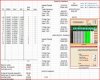
For each of the 100 completed simulations, I will report it’s hourly win-rate and will organize them moving from greatest to lowest (like the optimism of this organization?).
Results (this is just a list. If you'd like to see a graphical representation of the data, skip to the next link):
https://docs.google.com/viewer?a=v&pid=explorer&chrome=true&srcid=0B0cCldUn36hMMWJkZDM0N2YtZWIzOC00ZTBjLTkxNDctNTQ0ZGU1NWU2NmZi&hl=fr
Some Raw Stats:
Mean: 2.183 units per hour
Median: 2.170 units per hour
Minimum: 1.770 units per hour
Maximum: 2.530 units per hour
Here is a nice graphic summarizing the above data:
https://docs.google.com/viewer?a=v&pid=explorer&chrome=true&srcid=0B0cCldUn36hMNjU1MTU3ZTMtNjY5Ny00YzYwLTg0NDctNzFmMTFiMzczY2Y1&hl=fr
Conclusions:
I’ll leave that to you all.
Disclaimers:
The fluctuations that one might experience over 3,000,000 rounds are likely larger than depicted in this study for a few reasons. First of all, the game studied was a double-deck game. It is known that the ratio of win rate : Standard Deviation is significantly lower in shoe games than it is in double-deck games such as the one studied here. It may be unrealistic to assume that one can put in 30 hours per week at the DD tables for an extended period of time, for these games tend to be more uncommon than shoe games, and they tend to be watched a bit more closely by the pit. Because one would likely have to play the occasional shoe game, one’s lifetime win rate likely will have fluctuated away from their EV more greatly than this study may indicate.
Moreover, no one plays perfect. The strategy used in this study was HO2 with ASC, full-indices and quarter-deck resolution. If you try to implement a strategy this difficult, you WILL make an occasional “mistake,” however small or insignificant it may be. Mistakes tend to increase variance and / or lower your EV, neither of which is good for the counter.
Another reason that the typical counter can’t play perfect is the occasional need for cover. It is known that betting cover is quite pricey in terms of increasing variance and lowering EV, ESPECIALLY IN CASES WHERE ONE IS NOT GETTING VERY MANY ROUNDS PER SHOE (I.e., lower number of decks or more players at the table).
I could dabble on forever as to why one’s expected win rate will likely fluctuate even further than the study indicates, but I’d probably not mention anything that you’re not aware of.
Best,
SP
Last edited:
 :whip: